Some of the examples in the Software section used artificially-prepared mixes of spheres and another kind of particle, for the sake of obviousness. Here we will look at a real-world sample that consists of two classes of particles. In the typical raw image shown below, there are small round particles together with larger, more irregular objects. (All particle and thumbnail images are reduced by about 1/3 in the x and y dimension, in this presentation.)
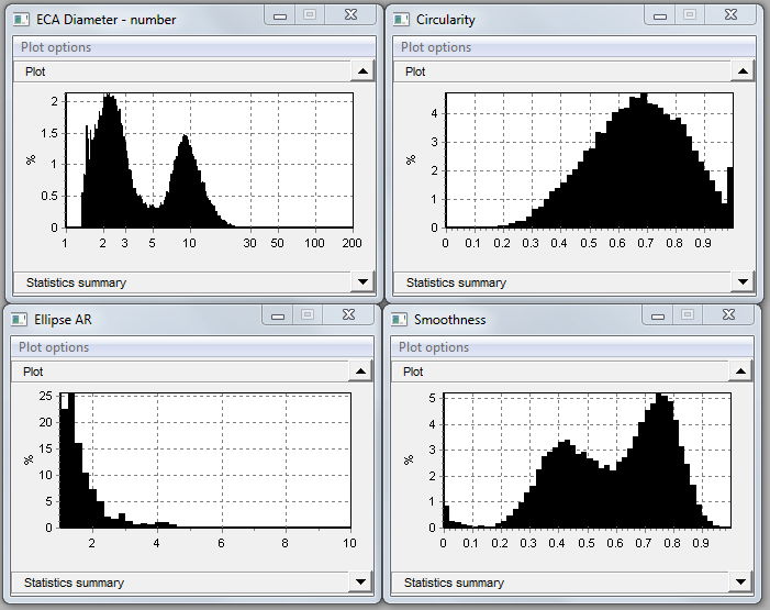
Above, we see frequency distributions for four measures, for this sample. The ECA diameter graph shows a bimodal distribution, probably representing the two kinds of particles observed in the raw image.
The task at hand is to extract separate size and shape statistics on the two sub-classes of particles. Three ways of accomplishing that task will be shown here.
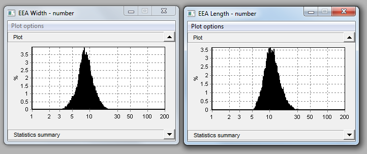
Before we start, note that the ellipse width and length graphs are almost identical, confirming that most of the particles have aspect ratio (length/width) close to 1. But that does not necessarily mean that they are spherical.
Single Measure Analysis
Below is the “large data window” for the ECA diameter. Also shown are statistics for the complete size range. The particle count is about 50,000, which is large enough to produce smooth distributions in the measure graphs. The dotted red lines indicate the likely overlapped parts of the two particle classes.
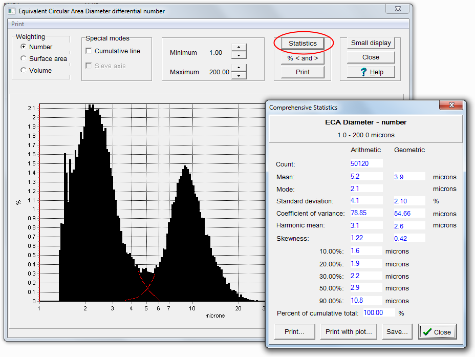 We can split the ECA distribution into two parts, to obtain a fairly good picture of the two classes of particles. Because of the overlap the two parts will each contain a small amount of data from the other size class. Below we close down the size range to that part of it that is below 5 microns, to isolate the first peak.

The smaller particles are seen to number about 31,000, and represent about 63% of the total, by number. The mean size is 2.5 microns and the median is 2.2 microns. The distribution is skewed slightly to the right (skewness > 0).
 In the graph above, we have restricted the size range to that part which is above 5 microns. These are the larger objects we see in the raw image. Particle count is about 18,000, representing 37% of the cumulative total by number. The Mean is 9.8 microns. Skewness shows as slightly positive, because the lower-end tail is cut off. In actuality, the distribution is probably pretty close to normal (unskewed).
This page of particle thumbnails for objects greater than 5 microns shows that they are irregular in shape.

Multi-measure Analysis
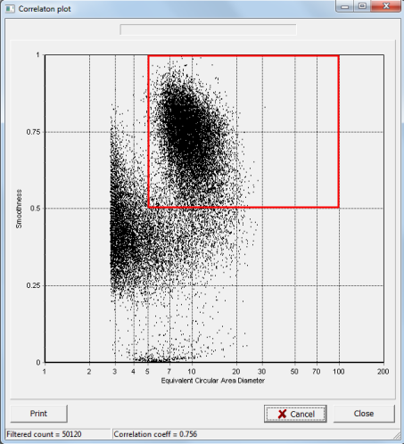
By taking into account other measures besides ECAD we may be able to separate the two particle classes more accurately. From the original Smoothness graph it looks like the two classes may have different smoothnesses. To confirm that, we can look at the correlation between ECAD and Smoothness:
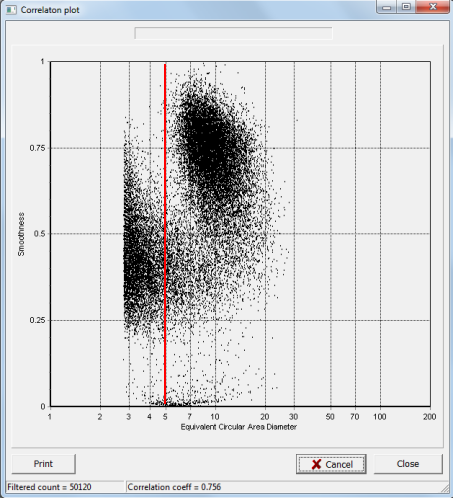
The two subpopulations show clearly in this scatter chart, although even here there is some amount of overlap. It is obvious from this chart that the larger class of particles are smoother on their surface than the smaller group. The red line represents the division of the sample into two parts that we did in the single-measure analysis. You can see that a fair number of “group 1” particles (the lower size group) actually got counted in group 2 in that method.
Is it possible to do a better job of separating the two parts? If you restrict ECAD to be > 5 and Smoothness to be > 0.5, then you take just the particles that are inside the red box below.
To do that, use the Particle Insight post-process reanalysis tool. Enter those restrictions in Limits:
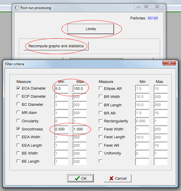
Click ‘Recompute graphs and statistics’ to regenerate all statistics. The resulting ECAD graph is probably pretty close to the actual size distribution in the upper group, and more accurate than simply taking the upper part of the original ECAD distribution.

Finding a rectangle that contains the lower size group is trickier, but ECAD < 8 microns and Smoothness < 0.6 catches most of them.
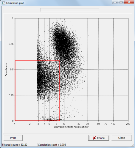
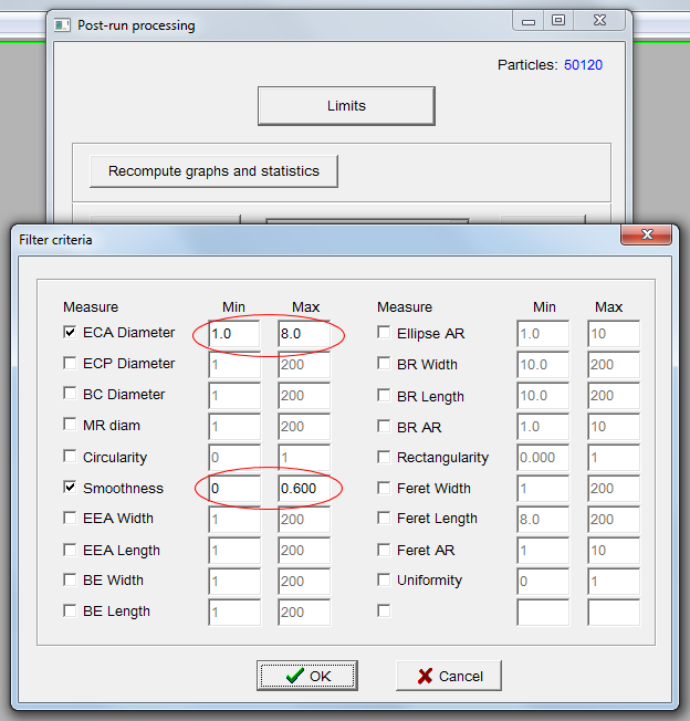
This class of particles is seen to be highly non-normal, with most particles at the low end. This is typical of very fine particles, both solid and liquid.
 There is a small overlap area that the two rectangles have in common, meaning that a few particles have been counted in both classes. But this technique does a reasonably good job of separating the classes, especially the group 2 (larger) class.
Particle Classification
The Classification tool in Post-Processing can do the same separation just described above, except that there are fewer steps. Define two classes as shown below:

Click OK, and a brief statistics summary is listed for each class:
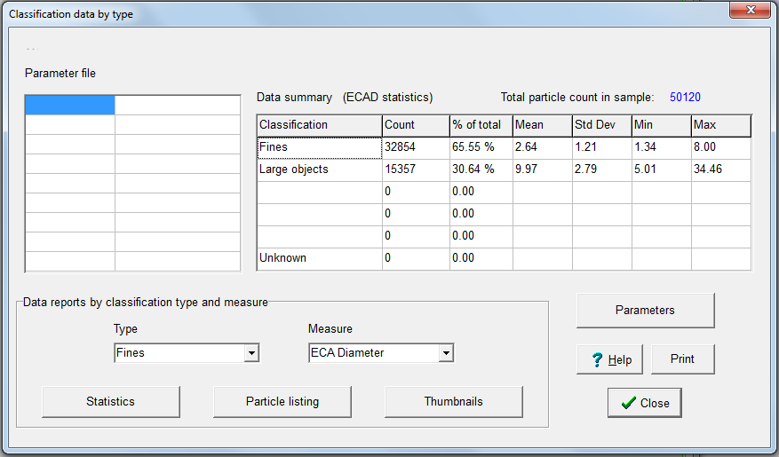
If I click Statistics, with Type equal to Fines, and Measure set to ECAD, I will get the same regeneration as I got before using ‘Recompute graphs and statistics’ for ECAD. To get results for the Large Objects class, just set Type to Large Objects and click Statistics again.
Further examples of these procedures can be found in the other application notes in this section.
Also see the video Separating subcomponents of a sample

