
Particle Basics
Basics of Particle Characterization
On this page
Particle characterization is the process of analyzing particles by particle shape, size, surface properties, charge properties, mechanical properties, microstructure and many more measurement parameters. There is a broad range of commercially available particle characterization techniques that can be used to measure particulate samples.
Size and shape are important attributes that affect the behavior of particulate substances. Spherical beads are easily and commonly characterized by a single size measure: “Diameter”. Irregular shapes are more difficult to characterize given their multi-dimensional structure. Powders used in manufacturing, for example, requires several measurement parameters to ensure flowability, packing and other performance functions.
Particle Size and Particle Shape Analysis are analytical techniques by which the distribution of sizes and shapes in a sample of particulate material is measured and reported. Particle size and particle shape analysis are an important tool in characterizing a wide range of final-product performance for quality control in many different industries, including paints, building materials, pharmaceutical, food industries and toners.
Statistical results are generally given with histograms of Because of the large number of particles, size and shape data are statistical. Histograms are the best way to portray statistical distributions of a variable or measure, and there are various means and measures of spread to characterize a distribution using just a few numbers.
Key Insight: Particle size measurements are highly dependent on particle morphology. Size-only techniques are suitable for spherical particles, but irregular particles require complementary shape analysis to ensure accurate characterization. Learn more about the impact of shape on size results →Particle shape impact particle size results using different techniques
Particle Size and Particle Shape are measures that greatly determine particulate behavior such as flowability, compaction, and mixing. Spherical particles are adequately characterized by size-only techniques. However, irregular particles require additional shape measurements to best characterize them and understand how your particles will perform.
Highly irregular shaped particles are hard to characterize, but for raw material particles in manufacturing, just knowing particle size is not enough. To truly understand particle behavior, it is required to measure more shape parameters and have tools that use these shape parameters to predict performance.
Dynamic image analysis is becoming more popular as a complementary analysis method because end users are beginning to understand the importance of large amounts of data for a large sample population. The first and most basic report of any particle size and particle shape analysis comes in the form of a statistical histogram.
- Distribution Histograms
To illustrate the statistical results from sample analysis, results are divided into small classes or “bins,” and the number of particles in each size bin is reported. Size information can be displayed in volume, number, and surface-area weighted histograms, each offering valuable information about the analyzed sample. Because dynamic image analysis is a number-based instrument, which means that each particle is identified and measured individually, the statistical histograms are very exact in each size bin. For example, in dynamic imaging systems users can easily view exactly how many particles are allocated in each of the size bins. Of course, since it’s an imaging system, the user can also see the individual particle thumbnail images that offer some objective evidence of what is being measured. Size data is usually depicted graphically on a log scale axis. Size and shape histograms are commonly used to compare differences in lots of samples.
Below are particle size histograms. Although they all may look different, these three histograms are of the same sample. Users should always view, at a very minimum, the number weighted distribution as well as the volume weighted distribution. Number weighted distributions are important for the user to view the presence of very fine particles in your sample. Very fine particles can impact a process where filtration can be clogged easily. In some cases, the presence of fine particles is important because they help lubricate the movement and flowability of particles. Therefore, there are different cases where fine particle presence can be a good thing or a bad thing. This is why number-weighted distributions should always be reviewed. Below you will also find a volume weighted statistical histogram. Volume weighted distributions are important to monitor large particle presence. Again, like fine particles, the presence of large particles may be wanted or undesirable. This is why viewing volume-weighted statistical distributions is also important. Surface area weighted distributions are sometimes used to gain an understanding of how much surface area a particle may have. However, there must be well understood that this is merely a calculation and does not take into consideration porosity. If your sample requires a more in depth understanding of surface area and porosity, it is recommended to look at equipment that can measure the specific properties. The last display of sieve equivalency is typically used for customers that have been using manual sieve measurements and are interested in converting to an automated method.
For more information on using Dynamic Imaging to replace Sieve analysis, please click here>> Sieve Correlation Using Dynamic Image Analysis
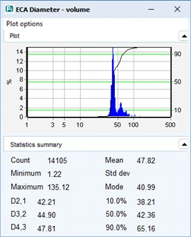
ECA Diameter — Volume Weighted
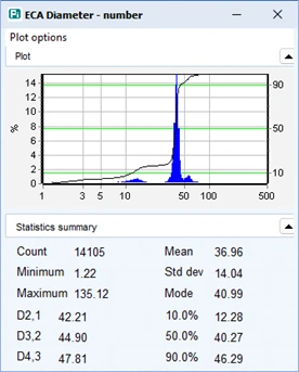
ECA Diameter — Number Weighted
Circularity, Smoothness & Aspect Ratio
In some cases, shape measurements are size-independent. In such cases, these fraction measures range from a value of zero to one. The following graph is a histogram showing a distribution of smoothness which is a measure of the irregularity in the perimeter of a particle. In this case the value of zero “0” would represent a very un-smooth particle and the value of one “1” would represent a very smooth particle. For practical use, a user could assume that the smoother a particle sample distribution is, the better the particles will flow. For more specific identification use a good example is to identify the non-smooth particles for metal powders in additive manufacturing where identification of non-smooth particles is necessary to ensure final product quality. There are many other fraction measurements for shape such as circularity, opacity, or aspect ratio. All of these are reported on a linear scale. Each bin reports its recorded quantity of particles.
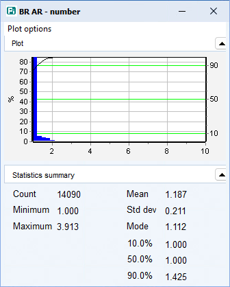
Also shown in a linear scale is aspect ratio. Shown below is bounding rectangle aspect ratio. Particle shape analyzers will typically have several different types of aspect ratio measurements. The user can select which aspect ratio measurement is more appropriate based on the shape of their particles. Aspect ratio measurements are typically between 1:00 and 10 but can be user defined. The bin spacing can also be user defined.
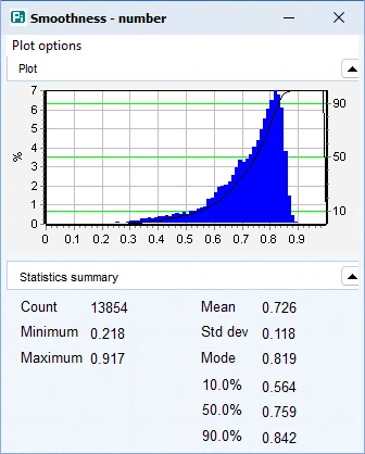
Smoothness Distribution
ECA Diameter — Number Weighted
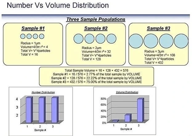
As discussed above, the reporting of number and volume-weighted distributions are very informative. Volume-weighted histograms will emphasize the presence of larger particles over the smaller ones, given the more significant volume larger particles have compared to a higher number of smaller ones. Volume-weighted histograms are helpful to identify small amounts of agglomerates in samples. Number-weighted histograms are helpful to identify large quantities of fine particles in samples, resulting in clogging or filtration issues. Of course, using dynamic image analysis, objective evidence of these particles are given in the form of thumbnail images of every measured particle: The following chart explains why one sample can have different number-weighted and volume-weighted histograms. This also shows the benefit of always studying both weighted statistics and using both to compare and contrast. The number and volume weighting can offer value in observing small quantities of agglomerates (larger particles) by reporting by volume and a higher number of fines (smaller particles) reporting by number.
Number vs. Volume Weighting
Volume-weighted histograms emphasize the presence of larger particles, while number-weighted histograms reveal large quantities of fine particles that may cause clogging or filtration issues. Both views are essential for thorough characterization.
Volume vs. Number Weighted Distributions
Sieve Users: For information on using Dynamic Imaging to replace sieve analysis, see Sieve Correlation Using Dynamic Image Analysis →>> Sieve Correlation Using Dynamic Image Analysis
- More on Statistics
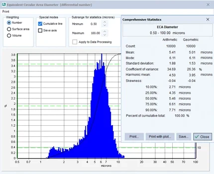
Equivalent Circular Area Diameter — Histogram & Statistics
A typical size distribution is characterized by different values. One of the most common being the mean size. A mean value allows some information of the particle size but does not issue any indication about the shape of the distribution or how broad or narrow it is. The number or arithmetic mean is purely the average value. It is frequently denoted as D1,0. Other means take into account volume weighting and area.
Assuming sphericity of particles, the generic definition of a weighted Dp,q mean diameter is
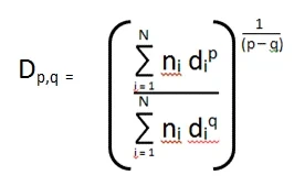
Weighted Dp,q Mean Diameter Formula
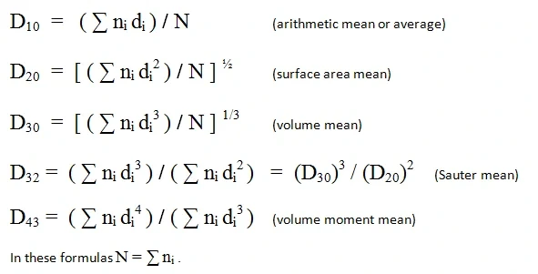
Dp,q Means Definitions
The Mode is the most frequent size present.
The Harmonic Mean is N / Σ (ni / di)
- Geometric Means
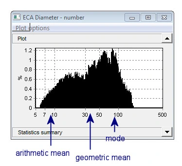
Arithmetic Mean, Geometric Mean & Mode
To compute the geometric mean, use the logs of the x-axis values ( log (di) in place of di ) :
Geometric Mean = Σ [ni · log(di)] / N
Measures of Spread
Standard deviation measures how wide the distribution is. The Coefficient of Variance is the ratio of the standard deviation to the mean: CV = σ / μ.
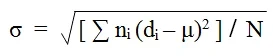
Standard Deviation Formula (μ = mean diameter D1,0)
- Percentiles
D10
10% of particles are smaller than this size
D50
The median — splits sample into two equal count halves
D90
90% of particles are smaller than this size
The 10th percentile represents the particle size below which 10% of the particle count falls. Other percentiles are defined in the same way. Commonly, the 10th, 50th, and 90th percentiles are used together to provide a simple yet more informative characterization than a single mean value. Additional percentiles can be calculated and customized within Insight software to meet specific industry requirements.
The volume median (50th percentile by volume) divides the total sample volume into two equal parts. While each portion contains the same volume, the number of particles in each may differ. Other volume percentiles follow the same principle; for example, the 25th volume percentile indicates the size below which particles account for 25% of the total sample volume.
- Other Characterizations
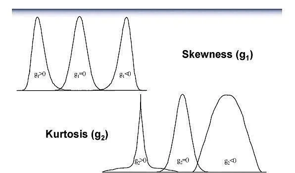
Skewness & Kurtosis
Skewness
An indicator of how asymmetrical the distribution shape is, about the center. A positive value means further counts on the right side (tail), while a negative value means it tails to the left.
Σ ni(di – μ)³ / (σ³ · N)
Kurtosis
An indicator of how much the shape differs from the typical bell curve in a vertical sense.
[Σ ni(di – μ)⁴ / (σ⁴ · N)] – 3
This article is also available on → AZoM.com